To machine learning engineers and data scientists, Jupyter notebooks have become a workhorse tool in the toolbox. Notebooks allow researchers to quickly prototype new solutions and make interactive visualizations in a remote computing environment. Unfortunately, the ease-of-use and interactivity of notebooks comes with some trade-offs when using version control.

Version control tools like git are powerful collaboration tools that track changes to source code and synchronize local and remote copies of a shared codebase. They allow developers to work together on the same codebase and seamlessly merge their improvements together. These tools also work out of the box with services like GitHub, which provide hosting for the shared codebase. Unfortunately, most of the user experience of using git and GitHub has been designed around text-based source code, but Jupyter notebooks are saved with embedded output media in a JSON format within .ipynb files.

As an example, let's imagine that we are quants at a new hedge fund called "Patagonia Capital". We decide it would be a good idea to create a repository to hold all of our exploratory data analysis (EDA) which will include shared Jupyter notebooks.

After completing this guide, you will learn how to:

• Setup auto-formatting in Jupyter notebooks
• Use VSCode's built-in tools for viewing notebook diffs
• Use nbstripout with git to only commit changes to notebook source
• Use papermill to create a shared library of executable notebooks
• And fetch some stock market data in Python!

After creating the "patagonia" Github repository for all the quants at Patagonia Capital, our next task is to setup the patagonia environment.

Tip #1: Auto-formatting in Jupyter notebooks

In our newly created repository, we can create the patagonia conda virtual environment. It's helpful to setup code formatting to provide some reasonable formatting standards across our company.

conda create -y -n patagonia python=3.8 
conda activate patagonia
conda install -y -c conda-forge pylint black jupyterlab jupyterlab_code_formatter

We can start jupyter lab to check that the code formatting is working. When you create a new notebook, you should see a Format notebook option in the notebook's toolbar.

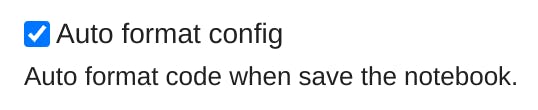
Since it's somewhat inconvenient to have to click the toolbar to perform code formatting, we can configure our formatter to format on save. Open up the Advanced Settings Editor via the Settings dropdown (or by pressing Cmd-, on Mac). Here, you will see the "Jupyterlab Code Formatter" settings for customization. At the bottom of these options, you can turn on the Auto format config checkbox.

Note: if you are using an older version of Jupyter, you may not see a checkbox for this setting. In this case, you can add the following under "User Preferences":

{
  "formatOnSave": true
}

When you return to your notebook, you should see that simply saving the notebook automatically formats your code. This will help make our changes easier to read within version control because our code will be committed with consistent formatting that is also designed to make diffs as small as they can be.

Tip #2: VSCode notebook diffs

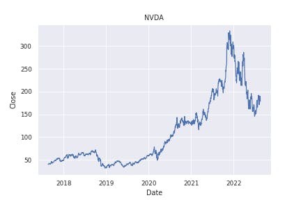
Now that we have our auto-formatting setup, let's plot the closing price of NVDA stock over the last 5 years. We'll first need to install some new dependencies.

conda install -y -c conda-forge pandas yfinance seaborn

Next, we can use Yahoo Finance along with Seaborn to make our plot of the NVDA ticker history in a Jupyter notebook:

# in plot_history.ipynb
import seaborn as sns
import yfinance as yf
from matplotlib import pyplot as plt

sns.set_theme("paper")

ticker = yf.Ticker("NVDA")
hist = ticker.history(period="5y")

plt.figure()
sns.lineplot(x="Date", y="Close", data=hist)
plt.savefig("NVDA_close_5y.png")
plt.show()

This will save the plot as a PNG image embedded in the notebook as well as in a new file called NVDA_close_5y.png. Since we're just getting started, let's imagine we directly commit this notebook and push it into the patagonia repository.

When we try to change something simple in our notebook like the ticker symbol from NVDA to AAPL, this is the diff we get in GitHub.

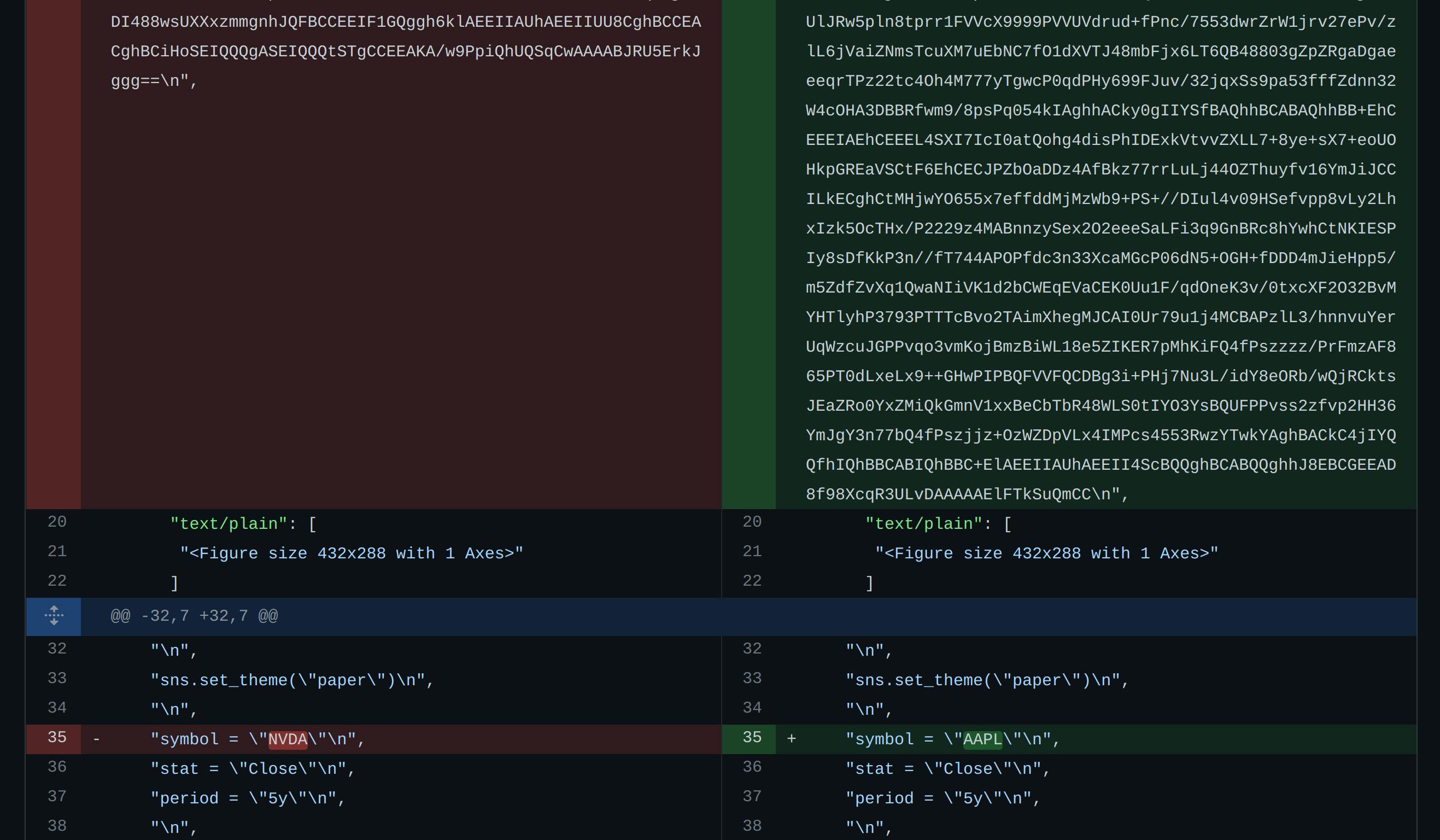
On the top, you can see the plot image changed (presumably both base-64 encoded). On the bottom, you can see the only change to the code, but it is inconveniently embedded in a string with escape characters.

If you were to look at the diff in VSCode, however, you would be pleasantly surprised to see this:

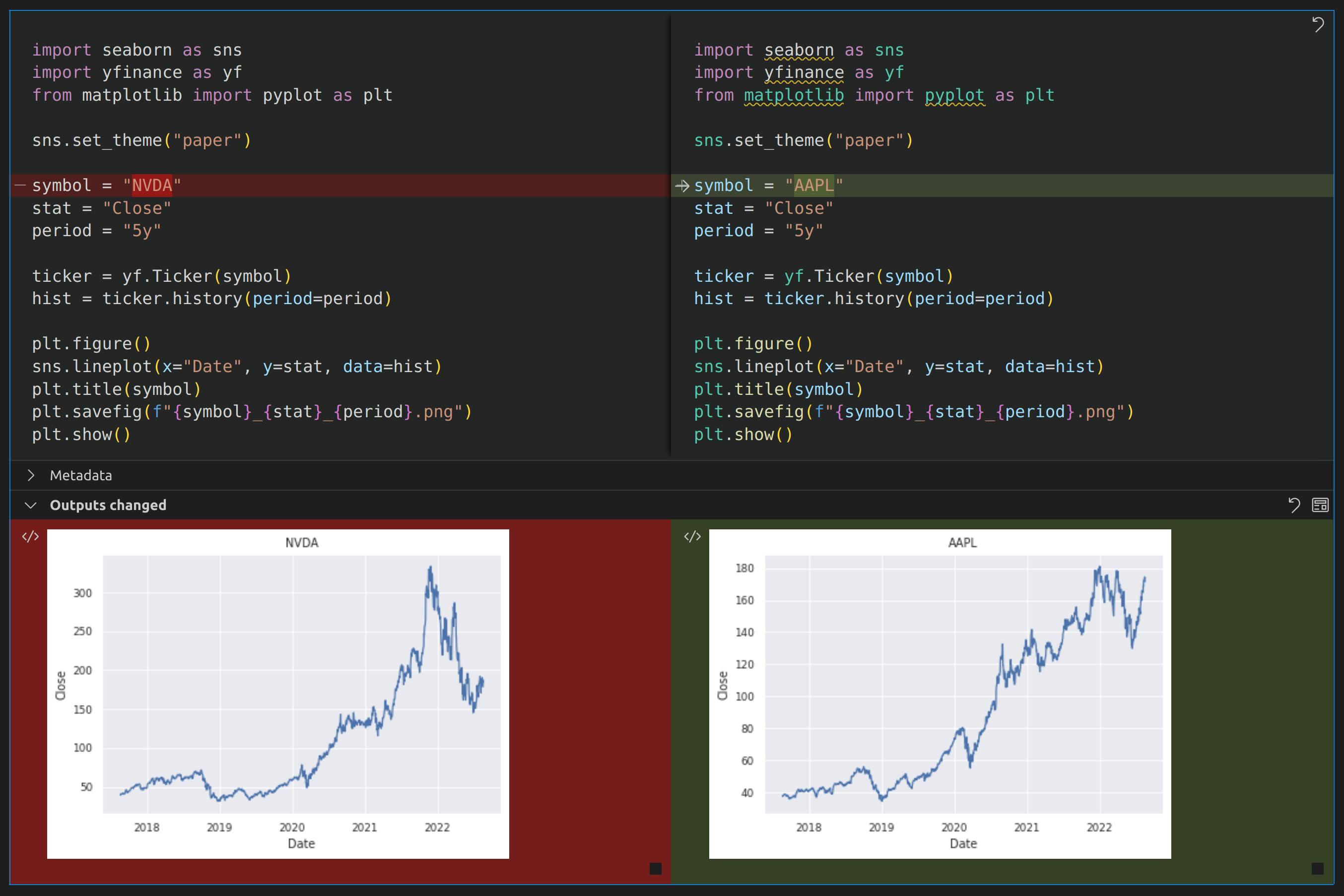
In VSCode, comparing different versions of Jupyter notebooks will show more informative diffs with your source code as well as changes in the rendered output.

Tip #3: nbstripout as git filter

Using auto-formatting and VSCode notebook diffs are really helping the devs at Patagonia Capital work togther, but sometimes we'd like to be a little more strict about what gets committed to our repository.

At Patagonia Capital, we've had some issues with new developers pushing massive notebooks to GitHub. To solve this type of problem, we can use nbstripout to automatically remove all notebook outputs before committing to our repository. To setup nbstripout, we need to do the following within our patagonia repository:

conda install -y -c conda-forge nbstripout
nbstripout --install --attributes .gitattributes

This will add a .gitattributes file (similar to a .gitignore file) which will tell git to apply the nbstripout filter to all .ipynb files. When this filter is applied to our notebooks, GitHub will no longer have the output plots.

If you'd like to automatically remove empty / tagged cells or retroactively apply this filter to your git history, you can read the nbstripout documentation on GitHub.

Tip #4: Executable notebooks with Papermill

While nbstripout has really helped Patagonia Capital avoid a bloated repository, we still sometimes would like to generate reports with standard visualizations from our growing library of notebooks.

Papermill allows running a Jupyter notebook as if it were an executable script. By designating certain cells as "parameters", papermill provides a command-line interface (CLI) to execute your notebooks and to specify parameter values via command-line arguments.

Let's install papermill and create an output/ folder for our "rendered" notebooks.

conda install -y -c conda-forge papermill
mkdir output

To avoid committing redundant rendered notebooks, we can add output/ to our .gitignore.

In Jupyterlab, we can bring our symbol, stat, and period constants to a separate cell. With that new cell active, we can open the Property Inspector and add a tag called "parameters":

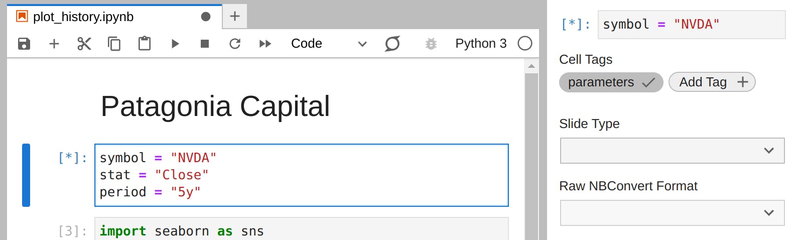
The values in this tagged cell will be default values to the notebook. We can execute our notebook to create a rendered notebook for the last 10 years of AAPL using the papermill CLI:

papermill plot_history.ipynb \
    output/plot_history_rendered.ipynb \
    -p symbol AAPL \
    -p period 10y

Papermill can also target cloud storage outputs for hosting rendered notebooks, execute notebooks from custom Python code, and even be used within distributed data pipelines like Dagster (see Dagstermill). For more information, see the papermill documentation.

Final thoughts

Jupyter notebooks and git are powerful tools for machine learning engineers and data scientists to prototype solutions and collaborate on a shared codebase. We discussed some tips and tricks for getting the best of both worlds from notebooks and version control in our simple financial example from Patagonia Capital.

Source availability

All source materials for this article are available here on my blog GitHub repo.